Modeling Airline Delay

Overview

Statistics on whether a flight was delayed and for how long are available from government databases for all the major carriers. It would be useful to be able to predict before scheduling a flight whether or not it was likely to be delayed. In this example, DataRobot will try to model whether a flight will be delayed, based on information such as the scheduled departure time and whether rained the day of the flight.

Prerequisites

In order to run this notebook yourself, you will need the following:

• This notebook. If you are viewing this in the HTML documentation bundle, you can download all of the example notebooks and supporting materials from Downloads.
• The datasets required for this notebook. These are in the same directory as this notebook.
• A DataRobot API token. You can find your API token by logging into the DataRobot Web User Interface and looking in your Profile.

Set Up

This example assumes that the DataRobot Python client package has been installed and configured with the credentials of a DataRobot user with API access permissions.

Data Sources

Information on flights and flight delays is made available by the Bureau of Transportation Statistics at https://www.transtats.bts.gov/ONTIME/Departures.aspx. To narrow down the amount of data involved, the datasets assembled for this use case are limited to US Airways flights out of Boston Logan in 2013 and 2014, although the script for interacting with DataRobot is sufficiently general that any dataset with the correct format could be used. A flight was declared to be delayed if it ultimately took off at least fifteen minutes after its scheduled departure time.

In additional to flight information, each record in the prepared dataset notes the amount of rain and whether it rained on the day of the flight. This information came from the National Oceanic and Atmospheric Administration’s Quality Controlled Local Climatological Data, available at http://www.ncdc.noaa.gov/qclcd/QCLCD. By looking at the recorded daily summaries of the water equivalent precipitation at the Boston Logan station, the daily rainfall for each day in 2013 and 2014 was measured. For some days, the QCLCD reports trace amounts of rainfall, which was recorded as 0 inches of rain.

Dataset Structure

Each row in the assembled dataset contains the following columns

• was_delayed
  • boolean
  • whether the flight was delayed
• daily_rainfall
  • float
  • the amount of rain, in inches, on the day of the flight
• did_rain
  • bool
  • whether it rained on the day of the flight
• Carrier Code
  • str
  • the carrier code of the airline - US for all entries in assembled dataset
• Date
  • str (MM/DD/YYYY format)
  • the date of the flight
• Flight Number
  • str
  • the flight number for the flight
• Tail Number
  • str
  • the tail number of the aircraft
• Destination Airport
  • str
  • the three-letter airport code of the destination airport
• Scheduled Departure Time
  • str
  • the 24-hour scheduled departure time of the flight, in the origin airport’s timezone

import pandas as pd
import datarobot as dr

data_path = "logan-US-2013.csv"
logan_2013 = pd.read_csv(data_path)
logan_2013.head()

	was_delayed	daily_rainfall	did_rain	Carrier Code	Date (MM/DD/YYYY)	Flight Number	Tail Number	Destination Airport	Scheduled Departure Time
0	False	0.0	False	US	02/01/2013	225	N662AW	PHX	16:20
1	False	0.0	False	US	02/01/2013	280	N822AW	PHX	06:00
2	False	0.0	False	US	02/01/2013	303	N653AW	CLT	09:35
3	True	0.0	False	US	02/01/2013	604	N640AW	PHX	09:55
4	False	0.0	False	US	02/01/2013	722	N715UW	PHL	18:30

We want to be able to make predictions for future data, so the “date” column should be transformed in a way that avoids values that won’t be populated for future data:

def prepare_modeling_dataset(df):
    date_column_name = 'Date (MM/DD/YYYY)'
    date = pd.to_datetime(df[date_column_name])
    modeling_df = df.drop(date_column_name, axis=1)
    days = {0: 'Mon', 1: 'Tues', 2: 'Weds', 3: 'Thurs', 4: 'Fri', 5: 'Sat',
            6: 'Sun'}
    modeling_df['day_of_week'] = date.apply(lambda x: days[x.dayofweek])
    modeling_df['month'] = date.dt.month
    return modeling_df

logan_2013_modeling = prepare_modeling_dataset(logan_2013)
logan_2013_modeling.head()

	was_delayed	daily_rainfall	did_rain	Carrier Code	Flight Number	Tail Number	Destination Airport	Scheduled Departure Time	day_of_week	month
0	False	0.0	False	US	225	N662AW	PHX	16:20	Fri	2
1	False	0.0	False	US	280	N822AW	PHX	06:00	Fri	2
2	False	0.0	False	US	303	N653AW	CLT	09:35	Fri	2
3	True	0.0	False	US	604	N640AW	PHX	09:55	Fri	2
4	False	0.0	False	US	722	N715UW	PHL	18:30	Fri	2

DataRobot Modeling

As part of this use case, in model_flight_ontime.py, a DataRobot project will be created and used to run a variety of models against the assembled datasets. By default, DataRobot will run autopilot on the automatically generated Informative Features list, which excludes certain pathological features (like Carrier Code in this example, which is always the same value), and we will also create a custom feature list excluding the amount of rainfall on the day of the flight.

This notebook shows how to use the Python API client to create a project, create feature lists, train models with different sample percents and feature lists, and view the models that have been run. It will:

• create a project
• create a new feature list (no foreknowledge) excluding the rainfall features
• set the target to was_delayed, and run DataRobot autopilot on the Informative Features list
• rerun autopilot on a new feature list
• make predictions on a new data set

Configure the Python Client

Configuring the client requires the following two things:

• A DataRobot endpoint - where the API server can be found
• A DataRobot API token - a token the server uses to identify and validate the user making API requests

The endpoint is usually the URL you would use to log into the DataRobot Web User Interface (e.g., https://app.datarobot.com) with “/api/v2/” appended, e.g., (https://app.datarobot.com/api/v2/).

You can find your API token by logging into the DataRobot Web User Interface and looking in your Profile.

The Python client can be configured in several ways. The example we’ll use in this notebook is to point to a yaml file that has the information. This is a text file containing two lines like this:

endpoint: https://app.datarobot.com/api/v2/
token: not-my-real-token

If you want to run this notebook without changes, please save your configuration in a file located under your home directory called ~/.config/datarobot/drconfig.yaml.

# Initialization with arguments
# dr.Client(token='<API TOKEN>', endpoint='https://<YOUR ENDPOINT>/api/v2/')

# Initialization with a config file in the same directory as this notebook
# dr.Client(config_path='drconfig.yaml')

# Initialization with config file located at ~/.config/datarobot/dr.config.yaml
dr.Client()

<datarobot.rest.RESTClientObject at 0x114014510>

Starting a Project

project = dr.Project.start(logan_2013_modeling,
                           project_name='Airline Delays - was_delayed',
                           target="was_delayed")
print('Project ID: {}'.format(project.id))

Project ID: 5c0012ca6523cd0200c4a017

Jobs and the Project Queue

You can view the project in your browser:

#  If running notebook remotely
project.open_leaderboard_browser()

True

#  Set worker count higher.
#  Passing -1 sets it to the maximum available to your account.
project.set_worker_count(-1)

Project(Airline Delays - was_delayed)

project.pause_autopilot()

True

#  More jobs will go in the queue in each stage of autopilot.
#  This gets the currently inprogress and queued jobs
project.get_model_jobs()

[ModelJob(Logistic Regression, status=inprogress),
 ModelJob(Regularized Logistic Regression (L2), status=inprogress),
 ModelJob(Auto-tuned K-Nearest Neighbors Classifier (Euclidean Distance), status=inprogress),
 ModelJob(Majority Class Classifier, status=inprogress),
 ModelJob(Gradient Boosted Trees Classifier, status=inprogress),
 ModelJob(Breiman and Cutler Random Forest Classifier, status=inprogress),
 ModelJob(RuleFit Classifier, status=inprogress),
 ModelJob(Regularized Logistic Regression (L2), status=inprogress),
 ModelJob(TensorFlow Neural Network Classifier, status=inprogress),
 ModelJob(eXtreme Gradient Boosted Trees Classifier with Early Stopping, status=inprogress),
 ModelJob(Elastic-Net Classifier (L2 / Binomial Deviance), status=inprogress),
 ModelJob(Nystroem Kernel SVM Classifier, status=inprogress),
 ModelJob(RandomForest Classifier (Gini), status=inprogress),
 ModelJob(Vowpal Wabbit Classifier, status=inprogress),
 ModelJob(Generalized Additive2 Model, status=inprogress),
 ModelJob(Light Gradient Boosted Trees Classifier with Early Stopping, status=queue),
 ModelJob(Light Gradient Boosting on ElasticNet Predictions , status=queue),
 ModelJob(Regularized Logistic Regression (L2), status=queue),
 ModelJob(Elastic-Net Classifier (L2 / Binomial Deviance) with Binned numeric features, status=queue),
 ModelJob(Elastic-Net Classifier (mixing alpha=0.5 / Binomial Deviance), status=queue),
 ModelJob(RandomForest Classifier (Entropy), status=queue),
 ModelJob(ExtraTrees Classifier (Gini), status=queue),
 ModelJob(Gradient Boosted Trees Classifier with Early Stopping, status=queue),
 ModelJob(Gradient Boosted Greedy Trees Classifier with Early Stopping, status=queue),
 ModelJob(eXtreme Gradient Boosted Trees Classifier with Early Stopping, status=queue),
 ModelJob(eXtreme Gradient Boosted Trees Classifier with Early Stopping and Unsupervised Learning Features, status=queue),
 ModelJob(Elastic-Net Classifier (mixing alpha=0.5 / Binomial Deviance) with Unsupervised Learning Features, status=queue),
 ModelJob(Auto-tuned K-Nearest Neighbors Classifier (Euclidean Distance), status=queue),
 ModelJob(Eureqa Generalized Additive Model Classifier (3645 Generations), status=inprogress),
 ModelJob(Naive Bayes combiner classifier, status=inprogress),
 ModelJob(RandomForest Classifier (Gini), status=inprogress),
 ModelJob(Gradient Boosted Trees Classifier, status=inprogress),
 ModelJob(Decision Tree Classifier (Gini), status=inprogress)]

project.unpause_autopilot()

True

Features

features = project.get_features()
features

[Feature(did_rain),
 Feature(Destination Airport),
 Feature(Carrier Code),
 Feature(Flight Number),
 Feature(Tail Number),
 Feature(day_of_week),
 Feature(month),
 Feature(Scheduled Departure Time),
 Feature(daily_rainfall),
 Feature(was_delayed),
 Feature(Scheduled Departure Time (Hour of Day))]

pd.DataFrame([f.__dict__ for f in features])

	date_format	feature_type	id	importance	low_information	max	mean	median	min	na_count	name	project_id	std_dev	target_leakage	time_series_eligibility_reason	time_series_eligible	time_step	time_unit	unique_count
0	None	Boolean	2	0.029045	False	1	0.36	0	0	0	did_rain	5c0012ca6523cd0200c4a017	0.48	FALSE	notADate	False	None	None	2
1	None	Categorical	6	0.003714	True	None	None	None	None	0	Destination Airport	5c0012ca6523cd0200c4a017	None	FALSE	notADate	False	None	None	5
2	None	Categorical	3	NaN	True	None	None	None	None	0	Carrier Code	5c0012ca6523cd0200c4a017	None	SKIPPED_DETECTION	notADate	False	None	None	1
3	None	Numeric	4	0.005900	False	2165	1705.63	2021	67	0	Flight Number	5c0012ca6523cd0200c4a017	566.67	FALSE	notADate	False	None	None	329
4	None	Categorical	5	-0.004512	True	None	None	None	None	0	Tail Number	5c0012ca6523cd0200c4a017	None	FALSE	notADate	False	None	None	296
5	None	Categorical	8	0.003452	True	None	None	None	None	0	day_of_week	5c0012ca6523cd0200c4a017	None	FALSE	notADate	False	None	None	7
6	None	Numeric	9	0.003043	True	12	6.47	6	1	0	month	5c0012ca6523cd0200c4a017	3.38	FALSE	notADate	False	None	None	12
7	%H:%M	Time	7	0.058245	False	21:30	12:26	12:00	05:00	0	Scheduled Departure Time	5c0012ca6523cd0200c4a017	0.19 days	FALSE	notADate	False	None	None	77
8	None	Numeric	1	0.034295	False	3.07	0.12	0	0	0	daily_rainfall	5c0012ca6523cd0200c4a017	0.33	FALSE	notADate	False	None	None	58
9	None	Boolean	0	1.000000	False	1	0.098	0	0	0	was_delayed	5c0012ca6523cd0200c4a017	0.3	SKIPPED_DETECTION	notADate	False	None	None	2
10	None	Categorical	10	0.053047	False	None	None	None	None	0	Scheduled Departure Time (Hour of Day)	5c0012ca6523cd0200c4a017	None	FALSE	notADate	False	None	None	17

Three feature lists are automatically created:

• Raw Features: one for all features
• Informative Features: one based on features with any information (columns with no variation are excluded)
• Univariate Importance: one based on univariate importance (this is only created after the target is set)

Informative Features is the one used by default in autopilot.

feature_lists = project.get_featurelists()
feature_lists

[Featurelist(Raw Features),
 Featurelist(Informative Features),
 Featurelist(Univariate Selections)]

# create a featurelist without the rain features
# (since they leak future information)
informative_feats = [lst for lst in feature_lists if
                     lst.name == 'Informative Features'][0]
no_foreknowledge_features = list(
    set(informative_feats.features) - {'daily_rainfall', 'did_rain'})

no_foreknowledge = project.create_featurelist('no foreknowledge',
                                              no_foreknowledge_features)
no_foreknowledge

Featurelist(no foreknowledge)

project.get_status()

{u'autopilot_done': False,
 u'stage': u'modeling',
 u'stage_description': u'Ready for modeling'}

# This waits until autopilot is complete:
project.wait_for_autopilot(check_interval=90)

In progress: 20, queued: 13 (waited: 0s)
In progress: 20, queued: 13 (waited: 1s)
In progress: 19, queued: 13 (waited: 1s)
In progress: 20, queued: 12 (waited: 2s)
In progress: 20, queued: 12 (waited: 4s)
In progress: 20, queued: 12 (waited: 6s)
In progress: 20, queued: 12 (waited: 10s)
In progress: 19, queued: 2 (waited: 17s)
In progress: 10, queued: 0 (waited: 30s)
In progress: 2, queued: 0 (waited: 56s)
In progress: 4, queued: 0 (waited: 108s)
In progress: 1, queued: 0 (waited: 198s)
In progress: 13, queued: 0 (waited: 289s)
In progress: 0, queued: 0 (waited: 379s)
In progress: 5, queued: 0 (waited: 470s)
In progress: 4, queued: 0 (waited: 560s)
In progress: 0, queued: 0 (waited: 651s)

project.start_autopilot(no_foreknowledge.id)

project.wait_for_autopilot(check_interval=90)

In progress: 0, queued: 0 (waited: 0s)
In progress: 0, queued: 0 (waited: 0s)
In progress: 0, queued: 0 (waited: 1s)
In progress: 0, queued: 0 (waited: 1s)
In progress: 0, queued: 0 (waited: 3s)
In progress: 0, queued: 0 (waited: 4s)
In progress: 0, queued: 1 (waited: 8s)
In progress: 20, queued: 13 (waited: 15s)
In progress: 20, queued: 1 (waited: 28s)
In progress: 3, queued: 0 (waited: 54s)
In progress: 16, queued: 0 (waited: 106s)
In progress: 20, queued: 12 (waited: 196s)
In progress: 0, queued: 0 (waited: 287s)

Models

models = project.get_models()
example_model = models[0]
example_model

Model(u'eXtreme Gradient Boosted Trees Classifier with Early Stopping and Unsupervised Learning Features')

Models represent fitted models and have various data about the model, including metrics:

example_model.metrics

{u'AUC': {u'backtesting': None,
  u'backtestingScores': None,
  u'crossValidation': 0.755494,
  u'holdout': 0.76509,
  u'validation': 0.75702},
 u'FVE Binomial': {u'backtesting': None,
  u'backtestingScores': None,
  u'crossValidation': 0.14855,
  u'holdout': 0.14992,
  u'validation': 0.15364},
 u'Gini Norm': {u'backtesting': None,
  u'backtestingScores': None,
  u'crossValidation': 0.510988,
  u'holdout': 0.53018,
  u'validation': 0.51404},
 u'Kolmogorov-Smirnov': {u'backtesting': None,
  u'backtestingScores': None,
  u'crossValidation': 0.398738,
  u'holdout': 0.42279,
  u'validation': 0.40472},
 u'LogLoss': {u'backtesting': None,
  u'backtestingScores': None,
  u'crossValidation': 0.272296,
  u'holdout': 0.27178,
  u'validation': 0.27079},
 u'RMSE': {u'backtesting': None,
  u'backtestingScores': None,
  u'crossValidation': 0.27529400000000004,
  u'holdout': 0.27627,
  u'validation': 0.27448},
 u'Rate@Top10%': {u'backtesting': None,
  u'backtestingScores': None,
  u'crossValidation': 0.379522,
  u'holdout': 0.35792,
  u'validation': 0.38908},
 u'Rate@Top5%': {u'backtesting': None,
  u'backtestingScores': None,
  u'crossValidation': 0.489794,
  u'holdout': 0.45902,
  u'validation': 0.5034},
 u'Rate@TopTenth%': {u'backtesting': None,
  u'backtestingScores': None,
  u'crossValidation': 0.8000019999999999,
  u'holdout': 0.75,
  u'validation': 0.66667}}

def sorted_by_log_loss(models, test_set):
    models_with_score = [model for model in models if
                         model.metrics['LogLoss'][test_set] is not None]
    return sorted(models_with_score,
                  key=lambda model: model.metrics['LogLoss'][test_set])

Let’s choose the models (from each feature set, to compare the scores) with the best LogLoss score from those with the rain and those without:

models = project.get_models()
fair_models = [mod for mod in models if
               mod.featurelist_id == no_foreknowledge.id]
rain_cheat_models = [mod for mod in models if
                     mod.featurelist_id == informative_feats.id]

models[0].metrics['LogLoss']

{u'backtesting': None,
 u'backtestingScores': None,
 u'crossValidation': 0.272296,
 u'holdout': 0.27178,
 u'validation': 0.27079}

best_fair_model = sorted_by_log_loss(fair_models, 'crossValidation')[0]
best_cheat_model = sorted_by_log_loss(rain_cheat_models, 'crossValidation')[0]
best_fair_model.metrics, best_cheat_model.metrics

({u'AUC': {u'backtesting': None,
   u'backtestingScores': None,
   u'crossValidation': 0.7132720000000001,
   u'holdout': None,
   u'validation': 0.71811},
  u'FVE Binomial': {u'backtesting': None,
   u'backtestingScores': None,
   u'crossValidation': 0.089814,
   u'holdout': None,
   u'validation': 0.09341},
  u'Gini Norm': {u'backtesting': None,
   u'backtestingScores': None,
   u'crossValidation': 0.426544,
   u'holdout': None,
   u'validation': 0.43622},
  u'Kolmogorov-Smirnov': {u'backtesting': None,
   u'backtestingScores': None,
   u'crossValidation': 0.322424,
   u'holdout': None,
   u'validation': 0.31053},
  u'LogLoss': {u'backtesting': None,
   u'backtestingScores': None,
   u'crossValidation': 0.291076,
   u'holdout': None,
   u'validation': 0.29006},
  u'RMSE': {u'backtesting': None,
   u'backtestingScores': None,
   u'crossValidation': 0.285848,
   u'holdout': None,
   u'validation': 0.28579},
  u'Rate@Top10%': {u'backtesting': None,
   u'backtestingScores': None,
   u'crossValidation': 0.294882,
   u'holdout': None,
   u'validation': 0.29352},
  u'Rate@Top5%': {u'backtesting': None,
   u'backtestingScores': None,
   u'crossValidation': 0.36734799999999995,
   u'holdout': None,
   u'validation': 0.39456},
  u'Rate@TopTenth%': {u'backtesting': None,
   u'backtestingScores': None,
   u'crossValidation': 0.600002,
   u'holdout': None,
   u'validation': 0.66667}},
 {u'AUC': {u'backtesting': None,
   u'backtestingScores': None,
   u'crossValidation': 0.7604420000000001,
   u'holdout': None,
   u'validation': 0.75549},
  u'FVE Binomial': {u'backtesting': None,
   u'backtestingScores': None,
   u'crossValidation': 0.15306999999999998,
   u'holdout': None,
   u'validation': 0.15124},
  u'Gini Norm': {u'backtesting': None,
   u'backtestingScores': None,
   u'crossValidation': 0.520884,
   u'holdout': None,
   u'validation': 0.51098},
  u'Kolmogorov-Smirnov': {u'backtesting': None,
   u'backtestingScores': None,
   u'crossValidation': 0.406068,
   u'holdout': None,
   u'validation': 0.39472},
  u'LogLoss': {u'backtesting': None,
   u'backtestingScores': None,
   u'crossValidation': 0.270848,
   u'holdout': None,
   u'validation': 0.27156},
  u'RMSE': {u'backtesting': None,
   u'backtestingScores': None,
   u'crossValidation': 0.274772,
   u'holdout': None,
   u'validation': 0.27497},
  u'Rate@Top10%': {u'backtesting': None,
   u'backtestingScores': None,
   u'crossValidation': 0.38498399999999994,
   u'holdout': None,
   u'validation': 0.38908},
  u'Rate@Top5%': {u'backtesting': None,
   u'backtestingScores': None,
   u'crossValidation': 0.504762,
   u'holdout': None,
   u'validation': 0.5034},
  u'Rate@TopTenth%': {u'backtesting': None,
   u'backtestingScores': None,
   u'crossValidation': 0.933334,
   u'holdout': None,
   u'validation': 1.0}})

Visualizing Models

This is a good time to use Feature Fit and Feature Effects (not yet available via the API) to visualize the models:

best_fair_model.open_model_browser()

True

best_cheat_model.open_model_browser()

True

Unlocking the Holdout

To maintain holdout scores as a valid estimate of out-of-sample error, we recommend not looking at them until late in the project. For this reason, holdout scores are locked until you unlock them.

project.unlock_holdout()

Project(Airline Delays - was_delayed)

best_fair_model = dr.Model.get(project.id, best_fair_model.id)
best_cheat_model = dr.Model.get(project.id, best_cheat_model.id)

best_fair_model.metrics['LogLoss'], best_cheat_model.metrics['LogLoss']

({u'backtesting': None,
  u'backtestingScores': None,
  u'crossValidation': 0.291076,
  u'holdout': 0.29408,
  u'validation': 0.29006},
 {u'backtesting': None,
  u'backtestingScores': None,
  u'crossValidation': 0.270848,
  u'holdout': 0.27193,
  u'validation': 0.27156})

Retrain on 100%

When ready to use the final model, you will probably get the best performance by retraining on 100% of the data.

model_job_fair_100pct_id = best_fair_model.train(sample_pct=100)
model_job_fair_100pct_id

'211'

Wait for the model to complete:

model_fair_100pct = dr.models.modeljob.wait_for_async_model_creation(
    project.id, model_job_fair_100pct_id)
model_fair_100pct.id

u'5c0016b76523cd026cc49f99'

Predictions

Let’s make predictions for some new data. This new data will need to have the same transformations applied as we applied to the training data.

logan_2014 = pd.read_csv("logan-US-2014.csv")
logan_2014_modeling = prepare_modeling_dataset(logan_2014)
logan_2014_modeling.head()

	was_delayed	daily_rainfall	did_rain	Carrier Code	Flight Number	Tail Number	Destination Airport	Scheduled Departure Time	day_of_week	month
0	False	0.0	False	US	450	N809AW	PHX	10:00	Sat	2
1	False	0.0	False	US	553	N814AW	PHL	07:00	Sat	2
2	False	0.0	False	US	582	N820AW	PHX	06:10	Sat	2
3	False	0.0	False	US	601	N678AW	PHX	16:20	Sat	2
4	False	0.0	False	US	657	N662AW	CLT	09:45	Sat	2

prediction_dataset = project.upload_dataset(logan_2014_modeling)
predict_job = model_fair_100pct.request_predictions(prediction_dataset.id)
prediction_dataset.id

u'5c0016cf6523cd0018c4a0d3'

predictions = predict_job.get_result_when_complete()

pd.concat([logan_2014_modeling, predictions], axis=1).head()

	was_delayed	daily_rainfall	did_rain	Carrier Code	Flight Number	Tail Number	Destination Airport	Scheduled Departure Time	day_of_week	month	positive_probability	prediction	prediction_threshold	row_id	class_0.0	class_1.0
0	False	0.0	False	US	450	N809AW	PHX	10:00	Sat	2	0.055054	0.0	0.5	0	0.944946	0.055054
1	False	0.0	False	US	553	N814AW	PHL	07:00	Sat	2	0.045004	0.0	0.5	1	0.954996	0.045004
2	False	0.0	False	US	582	N820AW	PHX	06:10	Sat	2	0.030196	0.0	0.5	2	0.969804	0.030196
3	False	0.0	False	US	601	N678AW	PHX	16:20	Sat	2	0.201461	0.0	0.5	3	0.798539	0.201461
4	False	0.0	False	US	657	N662AW	CLT	09:45	Sat	2	0.072447	0.0	0.5	4	0.927553	0.072447

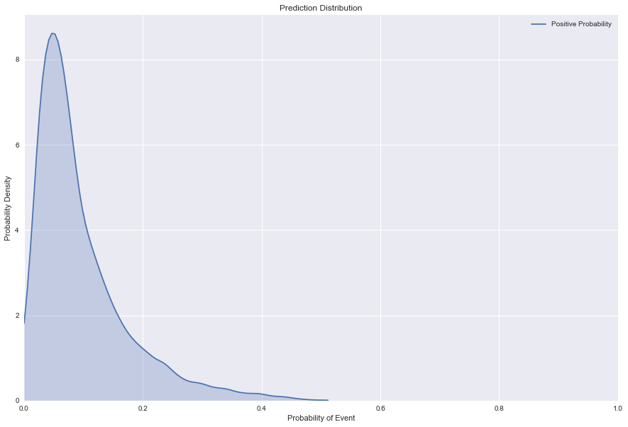
Let’s have a look at our results. Since this is a binary classification problem, as the positive_probability approaches zero this row is a stronger candidate for the negative class (the flight will leave on-time), while as it approaches one, the outcome is more likely to be of the positive class (the flight will be delayed). From the KDE (Kernel Density Estimate) plot below, we can see that this sample of the data is weighted stronger to the negative class.

%matplotlib inline
import seaborn as sns
import matplotlib.pyplot as plt
import matplotlib

matplotlib.rcParams['figure.figsize'] = (15, 10)  # make charts bigger

sns.set(color_codes=True)
sns.kdeplot(predictions.positive_probability, shade=True, cut=0,
            label='Positive Probability')
plt.xlim((0, 1))
plt.ylim((0, None))
plt.xlabel('Probability of Event')
plt.ylabel('Probability Density')
plt.title('Prediction Distribution')

Text(0.5,1,'Prediction Distribution')

---

Exploring Prediction Explanations

Computing prediction explanations is a resource-intensive task, but you can help reduce the runtime for computing them by setting prediction value thresholds. You can learn more about prediction explanations by searching the online documentation available in the DataRobot web interface.

When are they useful?

A common question when evaluating data is “why is a certain data-point considered high-risk (or low-risk) for a certain event”?

A sample case for prediction explanations:

Clark is a business analyst at a large manufacturing firm. She does not have a lot of data science expertise, but has been using DataRobot with great success to predict likely product failures at her manufacturing plant. Her manager is now asking for recommendations for reducing the defect rate, based on these predictions. Clark would like DataRobot to produce prediction explanations for the expected product failures so that she can identify the key drivers of product failures based on a higher-level aggregation of explanations. Her business team can then use this report to address the causes of failure.

Other common use cases and possible explanations include:

• What are indicators that a transaction could be at high risk for fraud? Possible explanations include transactions out of a cardholder’s home area, transactions out of their “normal usage” time range, and transactions that are too large or small.
• What are some explanations for setting a higher auto insurance price? The applicant is single, male, age under 30 years, and has received traffic tickets. A married homeowner may receive a lower rate.

Preparation

We are almost ready to compute prediction explanations. Prediction explanations require two prerequisites to be performed first; however, these commands only need to be run once per model.

Feature Impact

A prerequisite to computing prediction explanations is that you need to compute the feature impact for your model (this only needs to be done once per model):

%%time
feature_impacts = model_fair_100pct.get_or_request_feature_impact()

CPU times: user 25.4 ms, sys: 5.09 ms, total: 30.5 ms
Wall time: 11.3 s

Prediction Explanations Initialization

After Feature Impact has been computed, you also must create a Prediction Explanations Initialization for your model:

%%time
try:
    # Test to see if they are already computed
    dr.PredictionExplanationsInitialization.get(project.id,
                                                model_fair_100pct.id)
except dr.errors.ClientError as e:
    assert e.status_code == 404  # haven't been computed
    init_job = dr.PredictionExplanationsInitialization.create(
        project.id,
        model_fair_100pct.id
    )
    init_job.wait_for_completion()

CPU times: user 24.9 ms, sys: 5.16 ms, total: 30 ms
Wall time: 11 s

Computing the prediction explanations

Now that we have computed the feature impact and initialized the prediction explanations, and also uploaded a dataset and computed predictions on it, we are ready to make a request to compute the prediction explanations for every row of the dataset. Computing prediction explanations supports a couple of parameters:

• max_explanations are the maximum number of prediction explanations to compute for each row.
• threshold_low and threshold_high are thresholds for the value of the prediction of the row. Prediction explanations will be computed for a row if the row’s prediction value is higher than threshold_high or lower than threshold_low. If no thresholds are specified, prediction explanations will be computed for all rows.

Note: for binary classification projects (like this one), the thresholds correspond to the positive_probability prediction value whereas for regression problems, it corresponds to the actual predicted value.

Since we’ve already examined our prediction distribution from above, let’s use that to influence what we set for our thresholds. It looks like most flights depart on-time so let’s just examine the explanations for flights that have an above normal probability for being delayed. We will use a threshold_high of 0.456 which means for all rows where the predicted positive_probability is at least 0.456 we will compute the prediction explanations for that row. For the simplicity of this tutorial, we will also limit DataRobot to only compute 5 explanations for us.

%%time
number_of_explanations = 5
pe_job = dr.PredictionExplanations.create(
    project.id,
    model_fair_100pct.id,
    prediction_dataset.id,
    max_explanations=number_of_explanations,
    threshold_low=None,
    threshold_high=0.456
)
pe = pe_job.get_result_when_complete()
all_rows = pe.get_all_as_dataframe()

CPU times: user 4.1 s, sys: 131 ms, total: 4.23 s
Wall time: 22.4 s

Let’s cleanup the DataFrame we got back by trimming it down to just the interesting columns. Also, since most rows will have prediction values outside our thresholds, let’s drop all the uninteresting rows (i.e. ones with null values).

import pandas as pd
pd.options.display.max_rows = 10  # default display is too verbose

# These rows are all redundant or of little value for this example
redundant_cols = ['row_id', 'class_0_label', 'class_1_probability',
                  'class_1_label']
explanations = all_rows.drop(redundant_cols, axis=1)
explanations.drop(['explanation_{}_label'.format(i)
                   for i in range(number_of_explanations)],
                  axis=1, inplace=True)

# These are rows that didn't meet our thresholds
explanations.dropna(inplace=True)

# Rename columns to be more consistent with the terms we have been using
explanations.rename(index=str,
                    columns={'class_0_probability': 'positive_probability'},
                    inplace=True)
explanations

	prediction	positive_probability	explanation_0_feature	explanation_0_feature_value	explanation_0_qualitative_strength	explanation_0_strength	explanation_1_feature	explanation_1_feature_value	explanation_1_qualitative_strength	explanation_1_strength	...	explanation_2_qualitative_strength	explanation_2_strength	explanation_3_feature	explanation_3_feature_value	explanation_3_qualitative_strength	explanation_3_strength	explanation_4_feature	explanation_4_feature_value	explanation_4_qualitative_strength	explanation_4_strength
39	0.0	0.471055	Scheduled Departure Time	-2.208920e+09	+++	1.072288	day_of_week	Sun	++	0.455652	...	++	0.362867	Destination Airport	CLT	++	0.345914	Tail Number	N537UW	++	0.242375
392	0.0	0.478501	Scheduled Departure Time	-2.208920e+09	+++	1.072288	day_of_week	Sun	++	0.455652	...	++	0.362867	Destination Airport	CLT	++	0.345914	Tail Number	N536UW	++	0.272234
13043	0.0	0.465055	Scheduled Departure Time	-2.208920e+09	+++	1.202299	Tail Number	N194UW	++	0.416944	...	++	0.391831	day_of_week	Sun	++	0.286239	month	12	++	0.273073
13259	0.0	0.463182	Scheduled Departure Time	-2.208920e+09	+++	1.141272	Destination Airport	CLT	++	0.391831	...	++	0.373726	Tail Number	N563UW	++	0.321922	month	12	++	0.256552
13843	0.0	0.498733	Scheduled Departure Time	-2.208920e+09	+++	1.270218	Flight Number	586	++	0.440506	...	++	0.355779	Tail Number	N647AW	++	0.241246	day_of_week	Thurs	++	0.224909
...	...	...	...	...	...	...	...	...	...	...	...	...	...	...	...	...	...	...	...	...	...
18015	0.0	0.497778	Scheduled Departure Time	-2.208920e+09	+++	1.565999	month	7	++	0.809545	...	++	0.347827	Tail Number	N534UW	++	0.247029	day_of_week	Thurs	+	0.224909
18165	0.0	0.466710	Scheduled Departure Time	-2.208920e+09	+++	1.368628	month	7	++	0.368182	...	++	0.347827	Tail Number	N173US	++	0.314294	Flight Number	800	+	0.093169
18382	0.0	0.481914	Scheduled Departure Time	-2.208920e+09	+++	1.281047	Flight Number	586	++	0.440506	...	++	0.396207	day_of_week	Thurs	++	0.224909	Tail Number	N660AW	+	0.164530
18392	1.0	0.506051	Scheduled Departure Time	-2.208920e+09	+++	1.334738	month	7	++	0.424888	...	++	0.347827	Tail Number	N170US	++	0.280126	day_of_week	Thurs	++	0.224909
18406	1.0	0.511845	Scheduled Departure Time	-2.208927e+09	+++	1.357411	month	7	++	0.855629	...	++	0.676216	Scheduled Departure Time (Hour of Day)	17	++	0.455910	Destination Airport	CLT	++	0.344885

24 rows × 22 columns

Explore Prediction Explanations results

Now let’s see how often various features are showing up as the top explanation for impacting the probability of a flight being delayed.

from functools import reduce

# Create a combined histogram of all our explanations
explanations_hist = reduce(
    lambda x, y: x.add(y, fill_value=0),
    (explanations['explanation_{}_feature'.format(i)].value_counts()
     for i in range(number_of_explanations)))

explanations_hist.plot.bar()
plt.xticks(rotation=45, ha='right')

(array([0, 1, 2, 3, 4, 5, 6]), <a list of 7 Text xticklabel objects>)

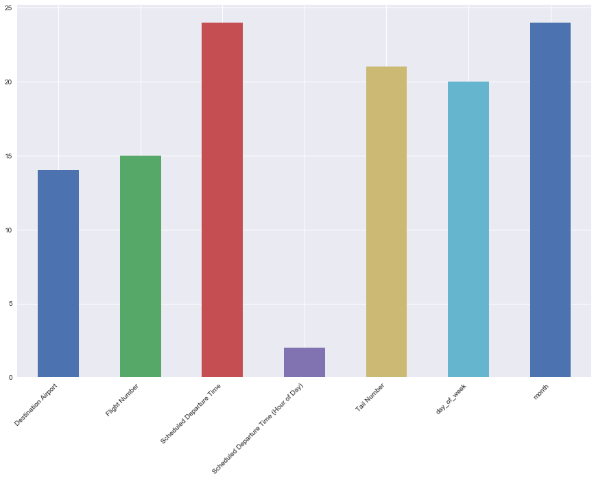
Knowing the feature impact for this model from the Diving Deeper notebook, the high occurrence of the daily_rainfall and Scheduled Departure Time as prediction explanations is not entirely surprising because these were some of the top ranked features in the impact chart. Therefore, let’s take a small detour investigating some of the rows that had less expected explanations.

---

Below is some helper code. It can largely be ignored as it is mostly relevant for this exercise and not needed for a general understanding of the DataRobot APIs

from operator import or_
from functools import reduce
from itertools import chain


def find_rows_with_explanation(df, feature_name, nexpls):
    """
    Given a prediction explanations DataFrame, return a slice
    of that data where the top N explanations match the given feature
    """
    all_expl_columns = (df['explanation_{}_feature'.format(i)] == feature_name
                        for i in range(nexpls))
    df_filter = reduce(or_, all_expl_columns)
    return favorite_expl_columns(df[df_filter], nexpls)


def favorite_expl_columns(df, nexpls):
    """
    Only display the most useful rows of a prediction explanations DataFrame.
    """
    # Use chain to flatten our list of tuples
    columns = list(chain.from_iterable((
        'explanation_{}_feature'.format(i),
        'explanation_{}_feature_value'.format(i),
        'explanation_{}_strength'.format(i))
        for i in range(nexpls)))
    return df[columns]


def find_feature_in_row(feature, row, nexpls):
    """
    Return the value of a given feature
    """
    for i in range(nexpls):
        if row['explanation_{}_feature'.format(i)] == feature:
            return row['explanation_{}_feature_value'.format(i)]


def collect_feature_values(df, feature, nexpls):
    """
    Return a list of all values of a given prediction explanation
    from a DataFrame
    """
    return [find_feature_in_row(feature, row, nexpls)
            for index, row in df.iterrows()]

---

Investigation: Destination Airport

It looks like there was a small number of rows where the Destination Airport was one of the top N explanations for a given prediction

feature_name = 'Destination Airport'
flight_nums = find_rows_with_explanation(explanations,
                                         feature_name,
                                         number_of_explanations)
flight_nums

	explanation_0_feature	explanation_0_feature_value	explanation_0_strength	explanation_1_feature	explanation_1_feature_value	explanation_1_strength	explanation_2_feature	explanation_2_feature_value	explanation_2_strength	explanation_3_feature	explanation_3_feature_value	explanation_3_strength	explanation_4_feature	explanation_4_feature_value	explanation_4_strength
39	Scheduled Departure Time	-2.208920e+09	1.072288	day_of_week	Sun	0.455652	month	2	0.362867	Destination Airport	CLT	0.345914	Tail Number	N537UW	0.242375
392	Scheduled Departure Time	-2.208920e+09	1.072288	day_of_week	Sun	0.455652	month	2	0.362867	Destination Airport	CLT	0.345914	Tail Number	N536UW	0.272234
13043	Scheduled Departure Time	-2.208920e+09	1.202299	Tail Number	N194UW	0.416944	Destination Airport	CLT	0.391831	day_of_week	Sun	0.286239	month	12	0.273073
13259	Scheduled Departure Time	-2.208920e+09	1.141272	Destination Airport	CLT	0.391831	day_of_week	Thurs	0.373726	Tail Number	N563UW	0.321922	month	12	0.256552
14226	Scheduled Departure Time	-2.208920e+09	1.339540	month	6	0.401657	Destination Airport	CLT	0.347827	day_of_week	Thurs	0.224909	Tail Number	N190UW	0.147016
...	...	...	...	...	...	...	...	...	...	...	...	...	...	...	...
17638	Scheduled Departure Time	-2.208920e+09	1.340564	month	7	0.411066	Destination Airport	CLT	0.347827	day_of_week	Thurs	0.224909	Flight Number	800	0.120877
18015	Scheduled Departure Time	-2.208920e+09	1.565999	month	7	0.809545	Destination Airport	CLT	0.347827	Tail Number	N534UW	0.247029	day_of_week	Thurs	0.224909
18165	Scheduled Departure Time	-2.208920e+09	1.368628	month	7	0.368182	Destination Airport	CLT	0.347827	Tail Number	N173US	0.314294	Flight Number	800	0.093169
18392	Scheduled Departure Time	-2.208920e+09	1.334738	month	7	0.424888	Destination Airport	CLT	0.347827	Tail Number	N170US	0.280126	day_of_week	Thurs	0.224909
18406	Scheduled Departure Time	-2.208927e+09	1.357411	month	7	0.855629	Tail Number	N818AW	0.676216	Scheduled Departure Time (Hour of Day)	17	0.455910	Destination Airport	CLT	0.344885

14 rows × 15 columns

all_flights = collect_feature_values(flight_nums,
                                     feature_name,
                                     number_of_explanations)
pd.DataFrame(all_flights)[0].value_counts().plot.bar()
plt.xticks(rotation=0)

(array([0]), <a list of 1 Text xticklabel objects>)

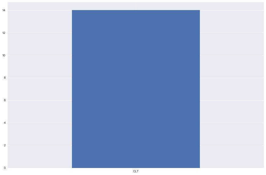
Many a frequent flier will tell you horror stories about flying in and out of certain airports. While any given prediction explanation can have a positive or a negative impact to a prediction (this is indicated by both the strength and qualitative_strength columns), due to the thresholds we configured earlier for this tutorial it is likely that the above airports are causing flight delays.

---

Investigation: Scheduled Departure Time

DataRobot correctly identified the Scheduled Departure Time input as a timestamp but in the prediction explanation output, we are seeing the internal representation of the time value as a Unix epoch value so let’s put it back into a format that humans can understand better:

# For simplicity, let's just look at rows where `Scheduled Departure Time`
# was the first/top explanation.
feature_name = 'Scheduled Departure Time'
bad_times = explanations[explanations.explanation_0_feature == feature_name]

# Now let's convert the epoch to a datetime
pd.to_datetime(bad_times.explanation_0_feature_value, unit='s')

39      1900-01-01 19:15:00
392     1900-01-01 19:15:00
13043   1900-01-01 19:10:00
13259   1900-01-01 19:10:00
13843   1900-01-01 19:15:00
                ...
18015   1900-01-01 19:10:00
18165   1900-01-01 19:10:00
18382   1900-01-01 19:15:00
18392   1900-01-01 19:10:00
18406   1900-01-01 17:05:00
Name: explanation_0_feature_value, Length: 24, dtype: datetime64[ns]

We can see that it appears as though all departures occurred on Jan. 1st, 1900. This is because the original value was simply a timestamp so only the time portion of the epoch is meaningful. We will clean this up in our graph below:

from matplotlib.ticker import FuncFormatter
from time import gmtime, strftime

scale_factor = 9  # make the difference in strengths more visible

depart = explanations[explanations.explanation_0_feature == feature_name]
true_only = depart[depart.prediction == 1]
false_only = depart[depart.prediction == 0]
plt.scatter(x=true_only.explanation_0_feature_value,
            y=true_only.positive_probability,
            c='green',
            s=true_only.explanation_0_strength ** scale_factor,
            label='Will be delayed')
plt.scatter(x=false_only.explanation_0_feature_value,
            y=false_only.positive_probability,
            c='purple',
            s=false_only.explanation_0_strength ** scale_factor,
            label='Will not')

# Convert the Epoch values into human time stamps
formatter = FuncFormatter(lambda x, pos: strftime('%H:%M', gmtime(x)))
plt.gca().xaxis.set_major_formatter(formatter)

plt.xlabel('Scheduled Departure Time')
plt.ylabel('Positive Probability')
plt.legend(markerscale=.5, frameon=True, facecolor="white")
plt.title("Relationship of Depart Time and being delayed")

Text(0.5,1,'Relationship of Depart Time and being delayed')

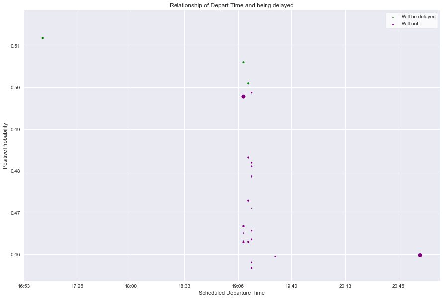
The above plot shows each prediction where the top influencer of the prediction was the Scheduled Departure Time. It’s plotted against the positive_probability on the Y-axis and the size of the plots represent the strength that departure time had on the prediction (relative to the other features of that given data point). Finally to aid visually, the positive vs. negative outcomes are colored.

As we can see by the time-scale on the X-axis, it doesn’t represent the full 24 hours; this is telling. Since we filtered our data earlier to only show predictions that were leaning towards being delayed, and this chart is leaning towards times in the afternoon and evening there may be a correlation between later scheduled departure time and a higher probability of being delayed. With a little bit of domain knowledge, one will understand that an airplane and its crew make many flights in a day (typically hopping between cities) so small delays in the morning compound into the evening hours.